Pure Python vs NumPy vs Sklearn Performance Comparison
By Heba Mohamed
- 8 minutes readTable of Content
BACKGROUND
Exaplination in depth the linear regression algorithm
Introduction
Linear regression algorithms show a linear relationship between a dependent $y$ and one or more independent $x$ variables, hence called linear regression.
Usage in real-word apps
Linear regression models have many real-world applications in an array of industries such as:
- Economics (e.g. predicting growth)
- Business (e.g. predicting product sales, employee performance)
- Social science (e.g. predicting political leanings from gender or race)
- Healthcare (e.g. predicting blood pressure levels from weight, disease onset from biological factors)
Important Assumptions in Regression Analysis
- Linearity: It is assumed that there is a linear relationship between the dependent $y$ and the independent $X$ variable(s).
- Autocorrelation: There should be no correlation between the residual (error) terms. If some correlation is present then it means that the model is unable to identify some relationship in the data.
- Multicollinearity: There should be no correlation between the independent variables. If the independent variables are moderately or highly correlated then it becomes difficult to find out which variable is contributing to predict the dependent (response) variable.
- Homoskedasticity: The error terms must have constant variance.This non-constant variance arises in the presence of outliers. When this phenomenon occurs, the confidence interval for the out of sample prediction tends to be unrealistically wide or narrow.
- Normality: The error terms must be normally distributed. Presence on non-normal distribution suggests that a few unusual data points must be studied closely to make a better model.
Note:
Mathematics Behind the Model
1. Simple Linear Regression
If a single independent variable (x) is used to predict the value of a numerical dependent variable (y). An estimate of this relationship is given as the linear function: $$yᵢ = β₀ + β₁Xᵢ + ε$$
Where:
- $y$ hat sub i $(ŷᵢ)$ represents the estimated output given the input.
- $Xᵢ$ In this equation, $β₀$ is a bias and $β₁$ is the weight of the model. If the model is charted so that the output is the y-axis and the input is the x-axis, $β₀$ refers to the $y$ - intercept and $β₁$ represents the slope.
- $ε$ represents the random error term. The random error term represents the residual error between an estimated relationship and the actual one. It is subject to variability.
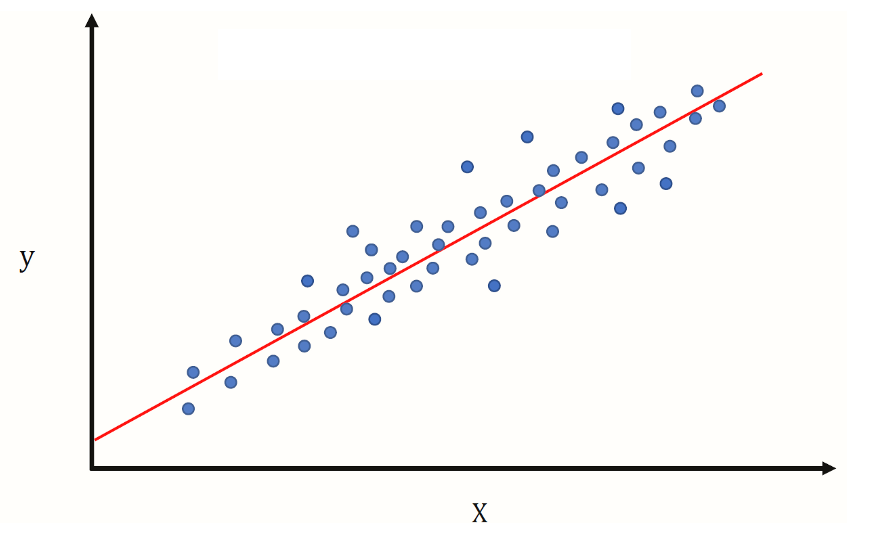
Simple linear regression data representation
2. Multiple Linear Regression
If more than one independent variable (X) is used to predict the value of a numerical dependent variable (y). An estimate of the relationship can be given as: $$ŷᵢ = β₀ + β₁Xᵢ₁ + β₂Xᵢ₂ + … βnXn + ε$$
Where:
- $Xᵢ₁, … Xᵢn$ represents all of the individual input datapoints where $Xᵢ₁$ represents a singular datapoint of input type $X₁$.
- $n$ is the number of input data types A multiple linear regression equation can be graphed as an n-dimensional plane.
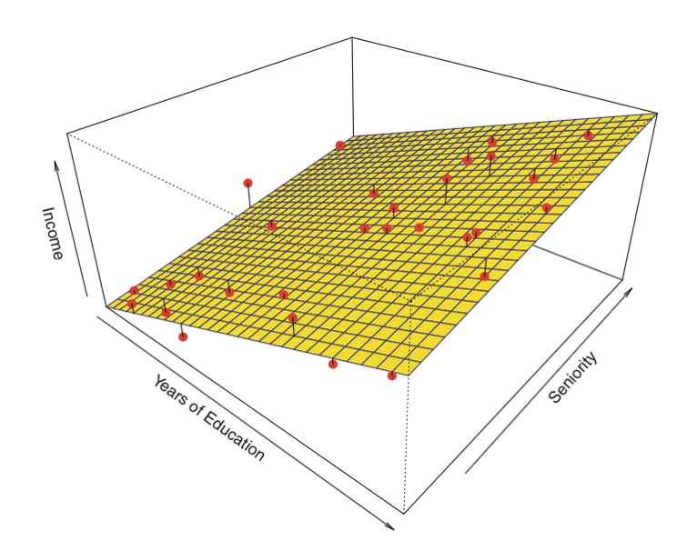
Example of n-dimensional plane
3. Minimize objective function for linear regression
The simple linear regression can be solved using Ordinary Least Squares (OLS), which is a statistical method, to find the model parameters.Our goal is to find statistically significant values of the parameters $β₀$ and $βn$ that minimise the difference between $y$ and $ŷ$.
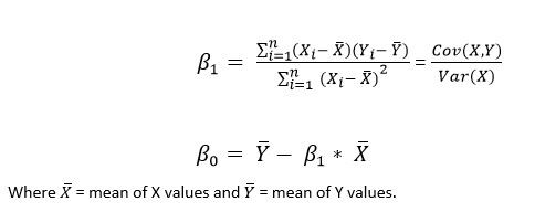
Ordinary Least Squares Single Linear Regression
4. Minimize objective function for multiple linear regression
We have more than one predictor variable which makes it hard for us to use that simple OLS method.we can implement a linear regression model for performing OLS regression using one of the following approaches
Note:
1. Solving the model parameters analytically (Normal Equations method)
This approach treats the data as a matrix and uses linear algebra operations to estimate the optimal values for the model parameters. It means that all of the data must be available and you must have enough memory to fit the data and perform matrix operations. So this method should be preferred for smaller datasets.
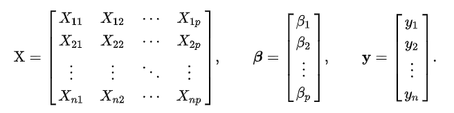
Ordinary Least Squares for Multiple Linear Regression
The closed-form solution for finding the optimal values for the model parameters is: $$Y = β^T.X$$ Finding the minimum can be achieved through setting the gradient of the loss to zero and solving for ${\beta}$ we get: $$β = (X^T.X)^-1X^T.Y$$
Note
2. Using an optimization algorithm (Gradient Descent, Stochastic Gradient Descent, etc.)
The general idea of Gradient Descent is to tweak parameters iteratively to minimize a cost function. Error/Cost here represents the sum of squared error between the predicted and the actual value. This error is defined in terms of a function and is called Mean Squared Error (MSE) cost function. So, the objective of this Gradient Descent optimization algorithm is to minimize the MSE cost function.
It measures the local gradient of the error function with regards to the parameter vector ${\beta}$ and it goes in the direction of the descending gradient. Once the gradient is zero, you have reached a minimum.
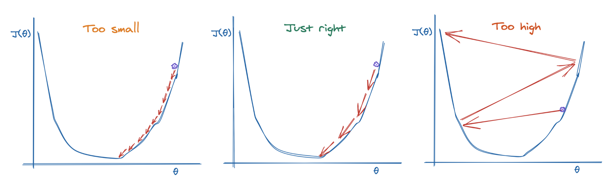
An important parameter in the Gradient Descent is the size of the steps, determined by the learning rate hyperparameter.
- If the learning rate is too small, the algorithm will have to go through many iterations to converge, which will take a long time.
- If the learning rate is too high, the algorithm will jump over the minimum, making it diverge. Hence the algorithm won’t reach the minimum.
Gradient desent optimization.
To implement the Gradient Descent, you need to compute the gradient of the cost function concerning the parameter vector ${\beta}$. To get the gradient, we need to take the partial derivative of the cost function.
The MSE cost function is defined as: $$MSE(β) = \frac{1}{m} \sum_{i=1}^{m} (y^{(i)} - β^T.X^{(i)})^2$$ $$\frac{\partial}{\partialβ_i}{MSE(β)}=\frac{2}{m}\sum_{i=1}^{m} (y^{(i)} - β^T.X^(i))X_{j}^{(i)}$$
Where:
- $m$ is the total number of observations (data points) $\frac{1}{m} \sum_{i=1}^{m}$ is the mean The vectorized form looks like $$\begin{split}\begin{align}∇_βMSE(β) = \begin{bmatrix} \frac{\partial}{\partialβ_0}{MSE(β)}\ \frac{\partial}{\partialβ_1}{MSE(β)}\ \text{.}\ \text{.}\ \frac{\partial}{\partialβ_n}{MSE(β)} \end{bmatrix} = \frac{2}{m} X^T.(X.β-Y)\end{align}\end{split}$$ The update rule to get the updated weights/parameters is given below: $$β^{(\text{next step})} = β - α\frac{\partial}{\partialβ_n}{MSE(β)} $$
Where:
- α is the learning rate hyperparameter.
PRACTICAL
Tools
- Python 3.
- Python basic modeules time, timeit, os, and itertools.
- NumPy Library (1.18.5).
- Matplotlib Library (3.3.2).
- Sklearn Library (1.0.1).
- Jupter Lab (3.2.5).
- Visual studio.
Proplem Specification
It is technically possible to implement scalar and matrix calculations using Python lists. However, this can be unwieldy, and performance is poor when compared to languages suited for numerical computation, such as MATLAB or Fortran, or even some general purpose languages, such as C or C++.
To circumvent this deficiency, several libraries have emerged that maintain Python’s ease of use while lending the ability to perform numerical calculations in an efficient manner. Two such libraries worth mentioning are NumPy (one of the pioneer libraries to bring efficient numerical computation to Python) and Sklrean (Simple and efficient tools for predictive data analysisSimple and efficient tools for predictive data analysis).
Although it is possible to use this deterministic approach to estimate the coefficients of the linear model, it is not possible for some other models, such as neural networks. In these cases, iterative algorithms are used to estimate a solution for the parameters of the model.
One of the most-used algorithms is gradient descent, which at a high level consists of updating the parameter coefficients until we converge on a minimized loss (or cost).
Create Dataset with Gaussian noise
This program creates a set of 10,000 inputs x linearly distributed over the interval from 0 to 2. It then creates a set of desired outputs $y = 3 + 2 * x + \text{noise}$, where noise is taken from a Gaussian (normal) distribution with zero mean and standard deviation sigma = 0.1.
- $X$: A set of 10,000 inputs from 0 to 2.
- $y = 3 + 2 * x + \text{noise}$
Note:
Model Using Pure Python
With a step size of 0.001 and 10,000 epochs, we can get a fairly precise estimate of $w_0$ and $w_1$. Inside the for-loop, the gradients with respect to the parameters are calculated and used in turn to update the weights, moving in the opposite direction in order to minimize the MSE cost function.
At each epoch, after the update, the output of the model is calculated. The vector operations are performed using list comprehensions. We could have also updated y in-place, but that would not have been beneficial to performance.
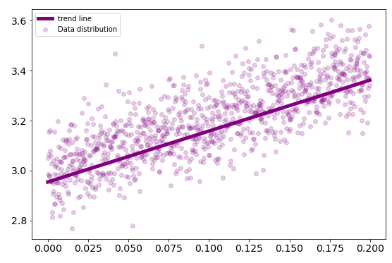
The elapsed time of the algorithm is measured using the time library. It takes $26.71$ seconds to estimate $w_0$ = 2.9657 and $w_1$ = 2.02859.
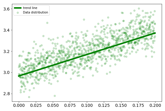
Best fitting line using pure python
Model Using NumPy Library
NumPy adds support for large multidimensional arrays and matrices along with a collection of mathematical functions to operate on them. I build a module called “MultipleLinearRegression” with the full implementation of linear regression algorithm using numpy.
The elapsed time of the algorithm is measured using the time library. It takes $0.9065$ seconds to estimate $w_0 = 2.9727$ and $w_1 = 2.02263$. While the timeit library provide $0.88965$ seconds.
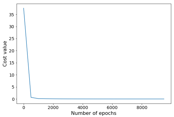
Error values vs number of epochs
Best fitting line using Numpy
Model Using Scikit-lwarn library
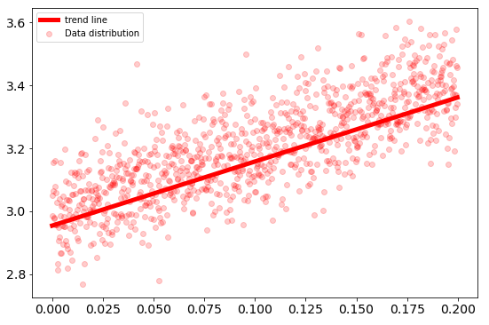
The elapsed time of the algorithm is measured using the time library. It takes $0.0009975433$ seconds to estimate $w_0 = 3.0015$ and $w_1 = 1.9982$. While the timeit library provide $0.00034485$ seconds.
Best fitting line using Scikit-learn
REFRENCES
- Least squares approximation
- Linear regression from ML cheatsheet
- Regression-metrics from machinelearningmastery
- Linear regression a complete story
- Introduction to linear regression in python
- Machine learning multivariate linear regression
- Numpy tensorflow performance from realpython
RESOUCES
- For more details see the project repository on github.
- Linear regression implementation modeule from here
- Dispaly the project notebook from here